The beat tracker your LED props deserve, a newly labeled 90 hour dataset, and TinyML that’s actually tiny.

I present to you the best beat tracker you can download right now, running on an RP2350 at 180MHz:

I really like flashy lights synched to music, and existing beat trackers are definitely pretty good and a lot of fun. I’m afraid though that “pretty good” LED cat ears don’t really cut it anymore in this economy, so here are the results of the last few months spent researching the topic.

Prior Art

The main projects that you can actually run and fit on a fast microcontroller are BTrack [6] (repo) and Michael Krzyzaniak’s Beat and Tempo Tracker, loosely based on [4] and [5].

Krzyzaniak’s BTT was the first one I found, and it’s a delightfully clear ANSI C library that just works and is super hackable. The gist of the method is:

• FFT over a window of audio samples, sum up the bins that increased from the previous window. This constitutes the “onset” signal.
• Compute the autocorrelation (AC) over a window of the onset signal. The highest candidate peaks are scored by cross-correlating them with a pulse train that combines common rythmic patterns.
• The AC lags with the best scores are accumulated in a histogram of recently observed tempos. The maximum of that histogram is taken as the current tempo.
• The current tempo/period is used in a kind of variable comb filter on the onset signal, emphasizing periodic peaks at the current tempo.
• Four pulses are cross-correlated with this recursive signal to determine the beat phase, which is then projected into the future to predict beats.

Now this works really well for how simple it is, the only issue is that it doesn’t really have memory to bridge sections where the beat signal is weak or absent. Once the last good beat leaves the 3 second buffer, we’re lost. This is also a strength, since it quickly adjusts to a new tempo or recovers when it loses tracking.

I’ve really tried, but could not manage to reliably lock onto a tempo and phase to carry the beat when the signal turns bad. For one, it’s quite difficult do determine when the beat strength signal is “good” or “bad”, without being either too conservative or too sensitive in switching from tracking the signal to projecting from the last good state. The other problem is that the beat strength signal just isn’t very good a lot of the time when there’s no nice transients on the beat, so phase detection using whatever Bayesian or other method you like is just wrong too often to be useful.

As this kind of machine grows, you end up stacking little box upon little box, each with a handful of weights, thresholds, hysteresis and inertia knobs to tune and it just gets out of hand. It always turns into the best kind of machine learning, where the machine is you and approximately zero learning happens.

Deep Learning Approach

Naturally there’s a bunch of papers solving beat tracking using trained models. For the most part, they’re built with a model that produces an activation function from audio input that’s used to estimate the parameters (period and phase) of a Hidden Markov Model (HMM) using Particle or Kalman Filters, full on Viterbi algorithm and more. So let’s try that!

The overall method is adapted from and a mix of Krebs et al. [3] that provides the HMM framework, BeatNet[1] and Don’t Look Back[2]. Honestly I didn’t look very deep into them, but on the surface they all seem similar. What mainly struck me was how massively all of them are limited by their training data, and conclusions and comparisons aren’t super interesting for the purpose of tracking dance music sets.

The largest datasets include Ballroom, Beatles, GTZAN, Carnatic and Rock and total to about 50 hours. Ballroom and GTZAN (14 hours) only contain 30 second clips, Beatles (8 hours) is only Beatles songs as the name suggests, leaving 13 hours of Rock Corpus and 16 hours of Carnatic music as full length songs by many artists.

I don’t know if that’s enough to really get close to the capacity of some of the (pretty sizeable) models used in the literature. In any case, these datasets aren’t going to get us very far for DnB or Zaagkicks. There isn’t anything else to download on Kaggle though, so what can you do :(

Jk, I built myself a little tool using my hands and brain, fired up yt-dlp and did some unpaid click work, almost making this a real AI project. Almost, because I got to listen to music I like instead of having to watch gore and CSAM videos for $2 a day.

So now I have 90 hours of meticulously annotated songs and live sets covering a good range of popular western pop and dancey music, with a focus on fast and harder styles. Glaring omissions that I can think of right now are Reggaeton and Dancehall. As far as I know that’s the largest dataset of annotated beats, not sure if I should be proud or worried.

But I’m not opposed at all to publishing it, in case people want to play with it or contribute (sample listing). Emphasis on people, because I’d prefer to know at least one or two humans are interested before letting the AI bots gobble it up. So just send an email :) but no creepy sentiment analysis and no GenAI!!

New Beat Tracking Model

A common choice of model from papers seems to be an LSTM with a few convolution layers to extract features from the input, which is usually some spectral representation like STFT outputs.

Now I’m not sure that LSTMs with 8 weight matrices each are the most parameter efficient choice to learn rythmic features, characterized by their multi-scale and kind of self similar nature. To me, the screams for a U-Net: stacked convolution blocks, first downsampling at each level so we go from full resolution to very coarse and then back up to “redistribute” the high level information to the needed granularity again.

And indeed the model I landed on is a small U-Net, currently with 18505 parameters. The input is audio at 16kHz sample rate through an STFT with window size 1024 and hop size 128 or 256, further shrunk into 64 Mel scale coefficients.

That’s a pretty stark contrast from papers where models get fed hundreds of coefficients derived from full CD quality audio, but I bet you can tap your foot to the sound leaking from other people’s earbuds on the bus, so why not expect the same from our model.

While I’m using Mel coefficients, the BeatNet[1] authors note that using learnable filters on the raw spectrum achieves “notably” better performance. I personally can’t confirm that, in my tests it made no difference either way, as did 99.99% of everything I tried.

The model is built entirely from depthwise separable 1d convolutions, first alternating between frequency and time convolutions in the frontend, and only temporal convolutions from then on in the U-Net blocks. In the bottleneck, the signal has been downsampled to 8Hz and is fed into a GRU cell with 24 hidden units. Then come the upsampling blocks with skip connections, and a fully connected layer to produce a single output.

The motivation for this extreme downsampling is that many challenging patterns are characterized by high level, large scale features. To be able to recognize anything like syncopation, snare rolls, dembow riddim, you need to listen for at least a few hundred milliseconds. There is no concept of rhythm at very small scale, and at larger scale rhythm by definition doesn’t change that quickly. Restating the same information hundreds of times per second is just wasted effort, and eliminating redundancy is what we’re after.

Nothing is causal, so the model actually works with a delay of 1.8 seconds, classifying the past so to say. In exchange it gets to look at 3.6 seconds of signal, so it has 1.8 seconds of context before and after the frame to classify. The reasoning for this is that at this scale, tempo has to be basically constant (Markovianity!) so information from 2 seconds ago is still relevant in the present. Also, you’re not really going to be doing inference in real-actually-real-time anyway and immediately react to the model’s output; in fact what you want is to predict beats, and then “react” to what you knew was coming long ago and have zero latency ideally. So why not, dropping causality makes the model’s task much easier and has few downsides for my purposes.

Channel counts are between 12 and 24, so the largest weight matrix has 576 entries. Some inner separable convolution blocks make use of GLU-like gating, where there’s two filters per input channel, and the output of one gets gated through the output of the second (\(out = out_1 \cdot \sigma(out_2)\)). I’ve shrunk this down as much as I was able to without losing performance, every component that remains has a measurable impact. Conversely that means that just making the model bigger doesn’t do very much, and I’ve also tried full Mobilenet blocks, ShuffleNet, nothing made much of a difference.

In fact the task is so easy on most of the data (80% is just kick drums), you can accidentally drop half of all channels, forget the sigmoid on the output logits, put a ReLU after the output unit, forget to pass in LSTM/GRU states, double log compress the model inputs and much more… And everything works well enough that it takes embarassingly long to notice.

Training

I used 60 second clips as training samples, with no augmentation for the time being. For labels, a gaussian with \(\sigma\approx 2\) is placed at beat positions. Because the inputs are small and the framerate low, we can backprop through half (sometimes all of) the sequence with 16GB of memory.

Everything has ended up being quite standard, binary cross-entropy loss with a weight of 8 for the positive class, Adam optimizer, gradient norm clipping and that’s it. More on the choice of loss function further down.

With batch size 128 on an RTX5080 (how are they so cheap to rent?), training converges in 4-5k steps, around 1h15m. There’s a bit of variation between runs, so trying a couple of initializations can be worth the time if you’re chasing decimal digits.

Implementation

The nice thing about a model with only two operators is that implementing it by hand is less code than the torch.export example notebook: we only need 1d convolution and matrix vector products because inference is done in a streaming manner, one sample at a time.

Each convolution layer has a ringbuffer to store its inputs. As soon as the input layer has pushed enough samples, we do the convolution to produce exactly one (1) output. The kernel doesn’t even move, it’s lovely.

Because of the progressive downsampling, most inputs don’t require much computation at all and only once every 2, 4, 8 samples it cascades down, like a marble machine counting in binary. This greedy strategy fails after the bottleneck though: because it’s upsampling, one value creates 2, 4, 8 outputs all by itself and every 8 steps we get a latency spike because we’re running the entire back half of the model. Unacceptable under realtime constraints.

The way to solve this problem in multirate systems is more buffering: instead of doing all the upsampling right away do only one step, keep the intermediate result and continue when the next input comes in. At the cost of a delay of 12 more frames for a total of 1.92 seconds, the worst case latency is back to manageable levels. The logic works out like this:

def on_sample():
  if try_down_0():
    # down_0 outputs every 2nd input
    if try_down_1():
      # down_1 outputs every 4th input
      if try_down_2():
        # down_2 outputs every 8th input
        # upsampling, so store 2 inputs for up_2
        enqueue_for_up_2()

  if t % 4 == 3:
    if try_up_2():
      enqueue_for_up_1()
  if t % 2 == 1:
    if try_up_1():
      enqueue_for_up_0()
  if try_up_0():
    output()

Tweaking the modulo conditions allows pairing up expensive down blocks with cheap up blocks and vice versa, to get the smoothest latency curve possible.

Particle Filtering

Particle Filters or Sequential Monte Carlo are used to estimate a the posterior distribution of the hidden states in a Markov process, in our case frequency \(f\) and phase \(\phi\) . Because this state space can be large (ours is not, really) it’s impractical to keep around density estimates at every possible state. So we limit the number of estimates in the form of a fixed number of particles with state \((f_i, \phi_i)\), each contributing to the estimate of posterior density at \((f_i, \phi_i)\) via its weight. The basic idea is to explore the state space with randomly spawned particles, and continuously evaluate how well the hypothesis represented each particle fits the incoming observations. If everything goes well, particles with high weight will end up concentrated around the true state.

The filter has a predict step where each particle can jump to a different state: in our model, that’s one step on the phase circle \(\phi_i^{t+1}=\phi_i^t + f_i \mod 1\), and a small probability of jumping to a different frequency.

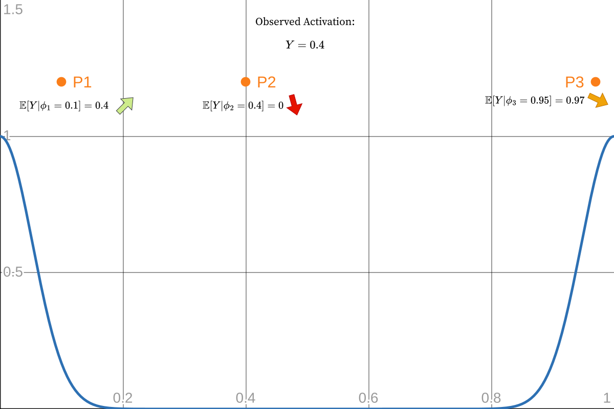
Then comes the update step where particles are judged against a new measurement, the model activation in our case. Each particle at \((f_i, \phi_i)\) has an expected prior distribution of activations: a big spike, around phase 0, and zero everywhere else. Given that prior, we compute the likelihood of the newly observed activation and update the weight.

I get confused with this stuff sometimes, so to make it clear we made this prior up. Obviously there’s reasons for picking this Gaussian and not any random shape but still, it remains arbitrary. At one point I had a little bump around \(0.5\) as well, because the model can have a higher activation on the offbeat as well. Allowing this offbeat activation makes the filter prefer slower tempos more often, so 90 instead of 180 bpm for example, which you may or may not want.

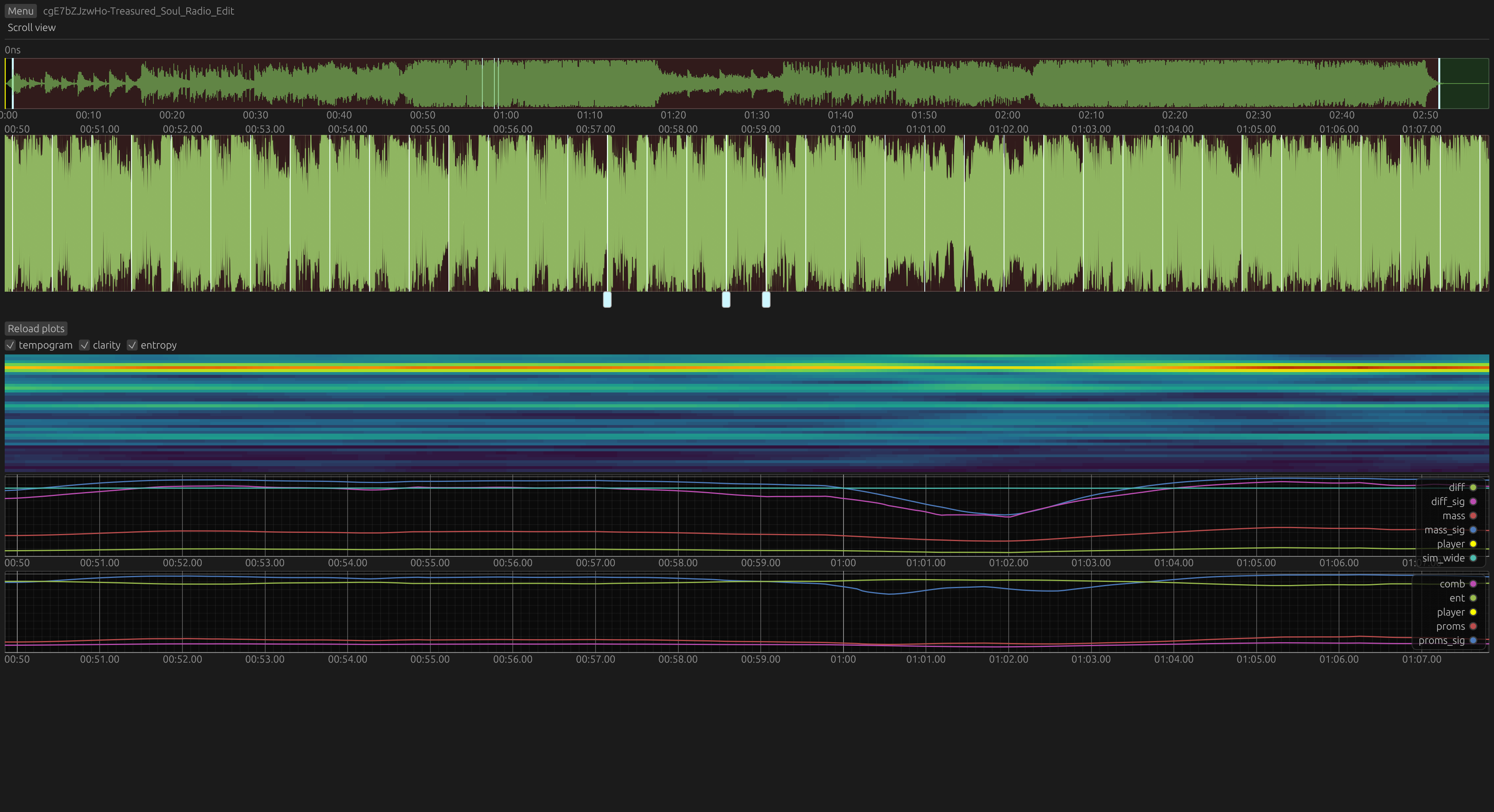
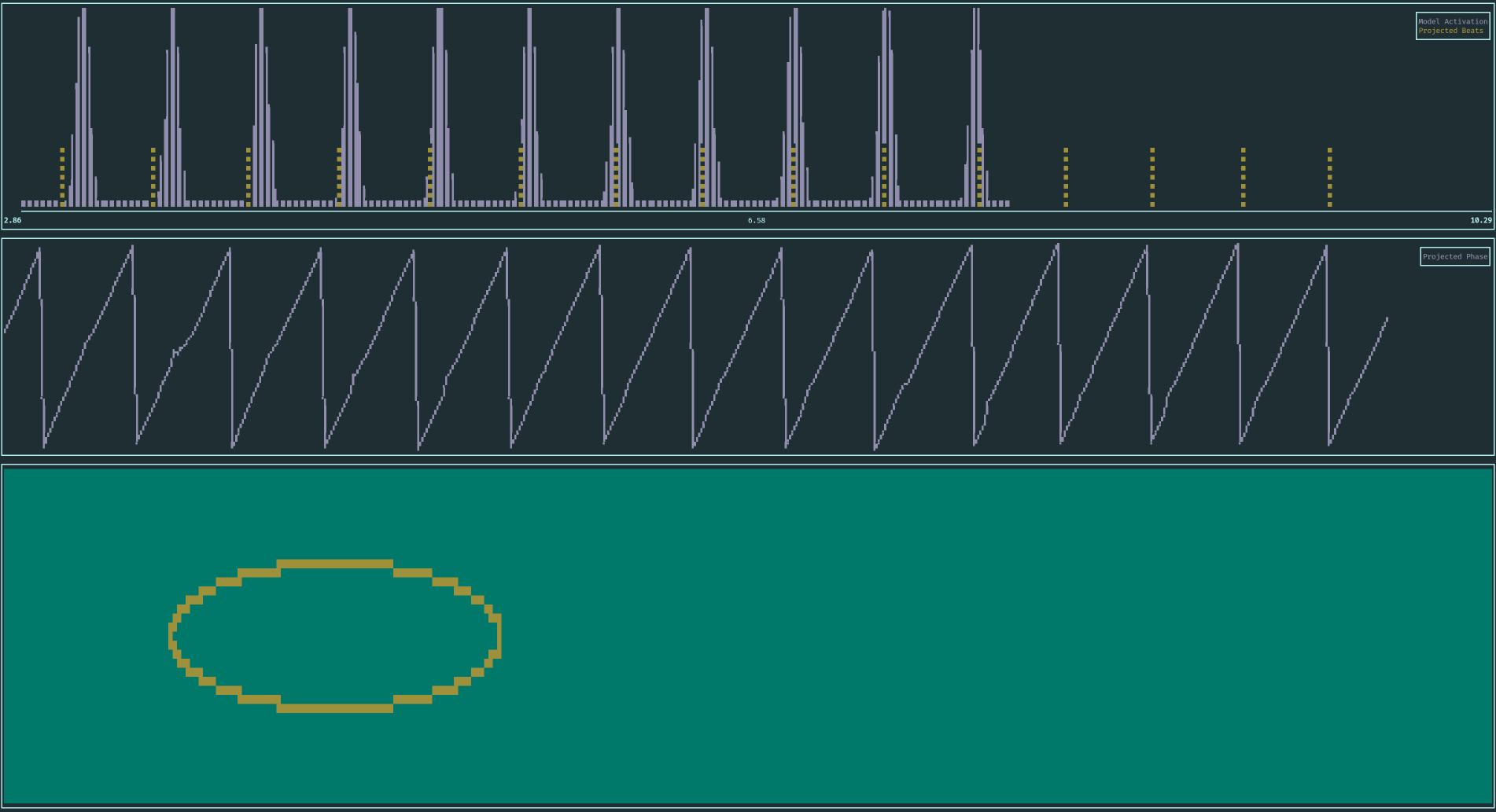
And here it is in action. Up top, particles moving through phase (X axis) and frequency/tempo (Y axis). The center plot shows the delayed model activation. At the bottom: particle filter phase in blue, phase projected into the present shown in red.

At the beginning, you can see roughly see all possible states. Also, notice the cluster at a slow tempo at first, then two at slow and fast tempo and finally the collapse to the fast cluster. Besides the cluster, a few particles are always injected to keep all tempo hypotheses alive and avoid getting stuck.

I mostly stuck to the mechanics described in [1, 2] with minor tweaks. The interesting and difficult part turns out to be the actual readout and how to produce discrete events from an evolving estimate of the phase posterior. For realtime readout, pretty much all choices are valid and will work: particle with the highest weight (MAP), weighted median phase, weighted average of phase using either trig functions or suitably unwrapping to handle the discontinuity at \(0\) and \(1\) all work when the particles are tightly clustered.

Projecting the current state into the future (actually present) is trickier: how phase evolves depends on the frequency (\(\phi = tf + C \mod 1\)), but we don’t have the phase and the frequency, only distributions. We can take expected values \(\mathbb{E}[f]\) and \(\mathbb{E}[\phi]\), sure, but not both: the delay we compensate through the projection is a fixed amount of time, not phase. And while \(t = \frac{\phi}{f}\) holds, \(\mathbb{E}[\frac{\phi}{f}]\ne \frac{\mathbb{E}[\phi]}{\mathbb{E}[f]}\), because \(\phi\) and \(f\) are very much not independent. You have to shift every particle by the required steps and then proceed.

None of this matters though when the cluster is tight and coherent with observations, everything works. We unwrap phase with the constraint that it can only move forwards, and when it crosses an integer that’s a beat.

Occasionally, often for short moments only, the cluster won’t be picture perfect but still present, and a little wiggle in the phase estimate causes a missed or spurious beat. Can we do something about that? After spending many days trying all kinds of approaches, my conclusion is that in practice you probably can’t. I’ll give some examples of why.

First observation: the sawtooth wave is nearly perfect, but around the beat when the new activation peak is coming in, particles are in the middle of being reweighted, some having seen the peak already while others are trailing behind and our phase estimate gets messed up at the last second. Could we instead accumulate evidence or belief over when the next beat will be in that clean portion, and then ignore what happens around the beat itself? Every particle \(i\) votes for \(\frac{1-\phi_i}{f_i}\) as the expected next beat time, and before some phase cutoff we freeze that estimate and consider it a beat. Maybe you can spot the problem: this quantity is only useful if all particles agree on which beat (in absolute time, seconds) we mean by the next one. Phase \(0.4\) can mean “I think beat \(k+1\) will occur \(\frac{0.4}{f_i}\) steps in the future” or “I don’t think beat \(k\) has even happened for another \(\frac{0.6}{f_i}\)”. Disambiguating is easy when the cluster is packed e.g., follow the best particle and it decides when the wraparound occurs. But the cluster isn’t perfect, that’s why we’re doing this in the first place! The best particle can be in very different places from one step to the next, so that’s no good.

That’s the problem at heart, unwrapping the phase circle into absolute time. My main ideas were:

• Emit two hypotheses for the next beat time, unwrapping assuming either “beat just happened” or “beat imminent”, and retrospectively score those predictions when new evidence arrives. Stick with the better one, and assume no phase slip happened in the meantime (kind of like beam search?)
• Straight up linear regression on past beats. Various flavours: regress both phase and frequency, or phase only with the PF estimate of frequency, or a mix of both, which I think makes it a sort of Phase Locked Loop (PLL). You can use that phase estimate as is, or only to disambiguate the unwrapping of the current PF state.

Those seem sound in theory, but none of it works in practice. By using the past to help interpret the present, we lose agility and temporal accuracy: a wrong call now is going to mess up the future as well. In the case of unwrapping phase into absolute time, mistaking beat \(k\) for beat \(k+1\) or assigning the wrong index (\(x\)) to a beat (\(y\)) will never correct itself and regressing \(y=mx+b\) will be forever wrong. So only look at a short window of the past and add some kind of sanity checks. If estimates are bad enough, reset everything and start again or whatever, we’re right back to stacking heuristics up to the ceiling.

Maybe you can improve tracking in terms of MSE, I don’t know. But perceived quality has suffered with everything I’ve tried: when the beat is clear and being snappy matters the most, MAP and co. are accurate, quick to adapt and quickly recover when the PF goes bad. But all of the “smart” systems are sticky to varying degrees, slow to recover and can rapidly oscillate between being early and late which is actually painful. Those are all (to me) way more noticeable than the occasional slipup.

And I forgot the most fun part! Phase isn’t the only circular thing, frequency is too! Averaging between 80 and 160 bpm makes no sense, those are just different views of the same hypothesis. So we fold everything into one tempo octave and are free to choose which harmonic to use. Here I gave the dominant harmonic some inertia, preventing erratic jumps between half and double tempo. Pick whichever, but stick with it for a while before switching again.

Fine, but what about that \(\frac{1-\phi}{f}\) time to next beat thing? A 80 bpm particle at \(\phi=0.25\) and 160 bpm at \(\phi=0.5\) both agree on the same beat grid. You can’t fold phase to lower frequencies though, how can the 160 bpm particle know if it’s the “one” or the “and” of the 80bpm quarter note… Sooo I guess fold phase to higher frequencies? In that case which half of the 80 bpm interval we were in actually helps to unwrap the 160 bpm phase, nice! But oh no, tempo being ambiguous and all, the 80 bpm cluster just jumped by half an interval, what does that mean for the 160 bpm particles? Did we move forwards or backwards in time? I don’t know, but by now the half tempo has disappeared, wait no there it is again. You get the point it just doesn’t work.

Evaluation

Evaluation was done with a 10 hour portion of my test set (159 single songs, missing the test excerpts of longer sets). Precision and recall are defined as predictions landing within 70, 35 and 10ms of the ground truth. For every method, the median deviation was subtracted from predictions because that’s very tunable and not an inherent weakness of any algorithm. There’s no special handling of half or double tempo errors, which is why there are small bumps around 50%. Cemgil score is also reported with \(\sigma = 40\text{ms}\), it’s akin to a gaussian error in the form \(\exp(\frac{-(x-\hat{x})^2}{2\sigma^2})\). Raw output here.

The PF uses 1500 particles, sampling 500 of them for the readout (that’s way more than needed, 800 to 1000 is plenty). BTT and BTrack are kept at their default settings, except for tempo limits. BTrack has a maximum tempo of 160 bpm hardcoded in a couple of places though, but simply changing that to 240 completely broke it so it’s a little bit at a disadvantage for some of the faster songs. As for the ML methods from the literature, honestly I can’t be bothered to repair more broken python projects right now, I’ve got enough of those myself lol. Without retraining on the same data, they might not be very good and with retraining they’ll likely end up pretty similar.

I’m very happy with these results, those median values mean match the perception that most pop songs and EDM that’s not uptempo-adjacent are pretty much perfect. The main goal was to be able to survive a pre-chorus, messy buildups to EDM drops and be on beat when the kick drum comes back, which has infinite potential for lighting effects. I think I’ve achieved that to a level I’m extremely happy with :)

Also turns out that even a hop size of 128 (so 125Hz) is more than is necessary, 256 works pretty much as well with half the computational cost. Since switching to double hop size I’ve also improved unrelated stuff which I’m not going to backport for one plot, so that’s why the 125Hz numbers are a bit worse.

You’ll notice the rightmost bars on the cemgil plot are missing at 62.5Hz, because with a 16ms granularity you just can’t be that precise. It’s probably not noticeable, 16ms is the equivalent of standing 5m away from the sound source. And in any case you might be able to mitigate this by not triggering on predicted beats themselves, but arming a super quick transient detector in a short window around them. I’d assume any delay is most noticeable when there’s prominent percussive sounds, so it might work.

Converting weights to float16 also doesn’t change performance, that’s an easy memory/cache win right there for supporting platforms.

Speed

The median time it takes to process 10 seconds of audio on my Ryzen 7840HS laptop:

• BTrack: 24ms, of which 19ms is the onset detection including FFT using KissFFT
• BTT: 409ms
• Mine: 25ms, of which 23ms is the model.

Both BTT and my Rust implementation use a textbook scalar FFT implementation, and BTT doesn’t really try to fast in any way. It also does a lot of work though, so I don’t know if it could be an order of magnitude faster.

The code is also still pretty simple, it’s just taking the easy way of doing way less work than the others. Nothing is really optimized on the small scale at this point.

On a Pico 2 RP2350 at 180MHz, eyeballed P99 latency is 15.3ms with P50 under 14ms. Cutting it close but has never missed the 16ms deadline yet. At 220MHz the maximum is around 12.2ms and median just under 10ms, so there’s time left to draw some LED animations without even using the second core!

Notes for the Future, What Didn’t Work

Non-Local Loss for Particle Filter Input

Earlier in this project, cross-entropy loss didn’t produce the results I expected. It was good, rock solid on easy parts but sometimes went completely off the rails when rhythm became less clear, messing up the particle filter that was supposed to bridge these very parts where the model is lost. My first idea was to introduce some simple and objective “difficulty” metric that would detect the most difficult sections in music. That could then be used to gate the model’s output and the loss, we’d effectively ignore these parts during training and mute the model at inference time. Doesn’t work, a simple metric like that doesn’t exist and the entire idea is probably a dead end. Every sentence like that is the executive summary of at least 3 days work by the way, not just a vague hunch.

The goal remains to teach the model to shut up when the signal is bad instead of erratic best effort outputs. BCE loss applies to binary classification problems, but is that really the task here?

Classification means to assign every frame a label, where all frames are scored independently and all equally important ¹. Assigning class 1 with probability \(0.7\) when it’s actually \(0.3\) is always penalized with the same loss, regardless of what’s around it.

In that sense our model is not really a classifier, instead it’s a sensor with the very specific task of making the particle filter produce the correct beats. So 0 and 1 are not really labels: 0 output means the PF just keeps coasting at the current tempo, and 1 does not directly result in a beat but rather means “strong evidence there is a beat here”, which the HMM reconciles with its current beliefs.

That thinking led me to a different scoring approach to capture a more fitting formulation of the model’s task: produce just enough confident peaks to make the PF do its job, and no more. False positives are always bad, but false negatives are not an issue provided there’s still enough spikes around to drive the PF. So the loss for one sample depends on the predictions and labels in a whole neighbourhood, which is definitely unusual. I couldn’t find any literature in this direction, but also don’t know what to search for.

The end result was this abomination of a loss function (\(\epsilon\), clamping etc. omitted for clarity):

def fn_penalty(probs: torch.Tensor, target: torch.Tensor):
    # Soft thresholding (optional, can kill gradients)
    thresh = 0.1
    k_thresh = 20.0
    probs = probs * torch.sigmoid(k_thresh * (probs - thresh))
    target = target * torch.sigmoid(k_thresh * (target - thresh))

    fn = F.relu(target - probs)
    # Convolution with a 3.3 seconds wide box filter (with smooth edges)
    window_size = int(3.3 * FRAME_RATE) # must be odd
    window_fn = local_avg(fn, window_size)

    # Subtract 0.7 to give a false negative budget that's penalized less
    cluster_pen = torch.exp(3 * (window_fn - 0.7)).clamp(0.01, 2.5)
    return (fn * cluster_pen).mean() * 100

def fp_penalty(probs: torch.Tensor, target: torch.Tensor):
    # beats around masks areas where there's no music/marked beats. Unclear what should happen there
    fp = F.relu(probs - target) * beats_around

    window_size = int(3.3 * FRAME_RATE)
    window_fp = local_avg(fp, window_size)

    allowed = 5 * one_target_bell / window_size

    cluster_pen = torch.exp(3 * (allowed - 1)).clamp(0.01, 3)
    return ((fp**2) * cluster_pen).mean()

The final loss is the sum of these two FN and FP terms. The main element is a weighting term of the form \(exp(\text{fn}_{window})\) that increases or decreases the weight of the local error depending on the average error around it. This allows us to give a sizeable false negative “budget” before the loss really increases. Interestingly being a bit more lenient with false positives also seems to help.

The formulation above is the result of a good number of experiments mostly by feel, there’s not much theoretical motivation behind it. A few other ways also worked, but the exponentials made for the most consistent training. The numbers are also largely made up, as it’s unclear what each of them does and getting statistically significant comparisons would require a lot of training runs. Changing any single parameter also changes the dynamics of the entire system, and FN and FP terms will settle in a different equilibrium that’s impossible to predict.

This non-local loss really did improve performance in the beginning, and qualitatively it’s still different now. In these badly aligned screenshots, the top graph is the output from a model trained with BCE, the bottom one with the custom loss.

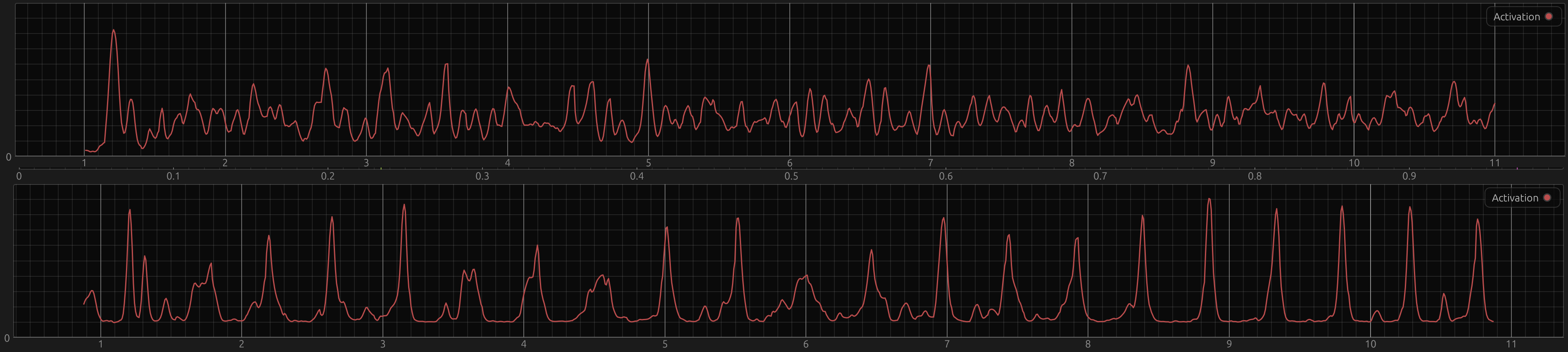
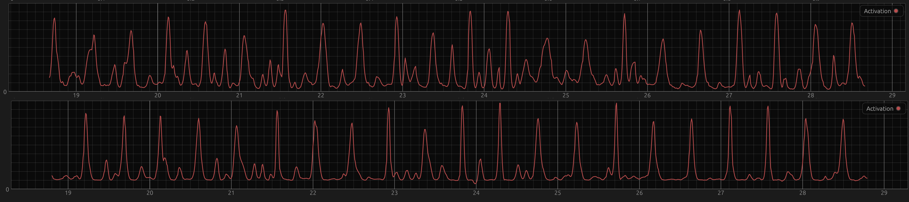
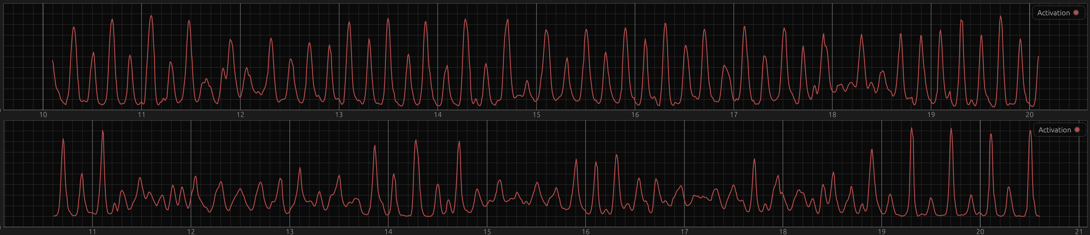
In general, the BCE model (top plots) has a higher noise floor and stays the same amplitude range and spikiness at the scale of ca. 10 seconds. The custom loss model in contrast can quite quickly switch from low amplitude to high peaks and back. When the signal is easy again, it’s almost like a different regime, where it’s beautiful peaks and then super flat again (sometimes with offbeat bumps), at 19s in the very bottom plot for example. With BCE, there’s always “more going on”.

As the dataset grew and the particle filter got better, the performance gap disappeared though, at least in terms of aggregate statistics. That doesn’t necessarily mean that they’re the same in terms of aesthetics and personal taste which retrieval metrics can’t capture. There’s no conclusion here, but it was interesting to me and might be worth pursuing.

Trainable HMM

Instead of training a model and hoping that it works with the particle filter or awkwardly taking turns optimizing the model and PF in EM fashion, you could also use a differentiable solution for the HMM and train everything end to end. Differentiable particle filters exist but seem really complicated. The state space is quite small though, on the order of \(10^{4}\) to \(10^{5}\), so just materializing the whole posterior distribution is very doable and at that point the math is pretty simple.

I’ve tried a little bit, nothing clever, torch.gather and scatter for the phase wraparound, log probabilities to make it work at all and that’s it. It kind of worked a little bit, but doing the loop over timesteps in Python is dog slow and 4 hours iteration time is not fun.

On that topic I also looked into Rao-Blackwellized particle filters, where each particle additionally keeps its own Kalman filter. It didn’t do a whole lot, but I also don’t know what advantages one would expect compared to the regular PF.

Even Smaller

Shrinking things even more will be more of a challenge, because just taking the current approach further noticeably impacts quality. The 16 ms hop size is starting to push it, unless you add interpolation in more places chopping beats into even coarser slices sounds rough. The particle filter does primitive \(2\times\) oversampling, without that a 180bpm interval only has 21 steps which is not a lot, at some point the PF dynamics might just not work anymore. The FFT window of 1024 samples is also near the limit, with 512 the spectrum really looks like garbage and the model doesn’t train nearly as well.

TODO

• Arduino and Micropython libraries!
• Decrease memory use: Model forward uses more scratch memory than necessary and never releases it between layers, and Particles don’t really need to be 3 floats.
• Maybe implement float16 weights, if it makes sense for any common MCU.
• Expose information about particle cluster quality, stop emitting beats when it’s bad.
• Gate model output? We only want spikes, constant activation is always wrong. A high pass filter or even a sort of transient detector might avoid make the PF more robust to erratic model outputs.
• Look into data augmentation again, my first attempt was too aggressive and got dropped at some point. But a tinny phone speaker currently makes tracking noticeably worse, so at least training on high pass filtered audio is a good idea.

That’s it :) The repo is here, there’s even a little TUI demo to play with that takes files or microphone input.

References