Fun with Local Image Features
Multi Kernel Descriptors, a different take on a DoG blob detector, and trying to make it all fast using Vulkan compute.
Introduction
Local Image Features are methods for finding and describing regions within an image such that regions human eyes can recognize as “similar” produce descriptors that are similar in a mathematical, quantifiable way.
The challenge in comparing images is that comparing millions of pixels is not only slow but also pointless, since two photos could look identical and have zero pixels of the same color in the same location. The common approach to solve this is to compress thousands of pixels into much fewer numbers that still capture the most important visual information, such that a small change in the input image only causes a small change in this descriptor. You can either do that for an entire image, or produce descriptors for many smaller patches within an image that only describe local features in the image.
Once you have a number of these descriptors from two images A and B, you try to match each descriptor in A to the most similar one in B. These point correspondences can be used for all kinds of tasks, such as camera or object tracking, image search engines, image stitching for satellite imagery, astrophotography and many more.
I’ve spent a good while researching and experimenting with more recent contributions in this little field, and this post is my selection of interesting things I’ve learned along the way. It’s also a high level intro to the topic for anyone who might be interested in it to get a feel for the methods and math involved, and how some really impressive looking tech starts as the composition of dead simple constructs.
Acknowledgements
- The work in this post originally started as my master’s thesis under the supervision of Prof. Voloshynovskiy at the University of Geneva. Almost everything presented here was done in my free time after that, and the implementation has largely been replaced since then. No affiliation, endorsement or review, this is just a random blog post.
- Vulkano (a Rust Vulkan wrapper) is one of the best pieces of software I’ve seen, and the recent taskgraph compiler and resource management are serious cutting edge stuff.
- Mesa AMD drivers are great, and capturing RGP profiles has not once crashed one me, unlike on Windows.
The Scale Invariant Feature Transform[8] by Lowe around 2000 was arguably the breakthrough method in this field, and is arguably still one of the best starting points for many tasks. It’s simple, mostly good enough to this day and super fast to compute. The Anatomy of the SIFT Method[10] provides a fantastic and digestible overview that I highly recommend, since my overview here is very crude and informal.
Step one in local feature extraction is to find those “salient features”, which just means stuff that stands out in an image. The type of feature that SIFT detects is called a blob and is exactly what it sounds like, a splotch of light or dark described by it’s location \((x, y)\) and a scale or radius \(\sigma\). That scale is important for the “Scale Invariant” part of SIFT: to match a large feature to the same one in another image where it’s further away and smaller, we need to know the size of both to isolate a patch around them and compute descriptors over only that feature.
A basic blob detector can be built from the Difference of Gaussians filter, a convenient approximation of the Laplacian of Gaussian filter, with appropriate low pass filtering as a bonus.
We start off by applying an increasingly large Gaussian blur filter to the image like so:

Intuitively, the scale of a blob corresponds to the blur level at which it disappears. To do that, we subtract each blur level from the next one to obtain the Difference of Gaussian (DoG) images. Consider these slices of a function with three inputs \(D(x, y, \sigma)\) that returns the response of a DoG filter of size \(\sigma\) at location \((x, y)\). What we’ve built is called a scale space representation of the image, and local extrema (a location and scale \((x, y, \sigma)\) marking a peak or valley in the DoG function) correspond to blob-like features.

We collect all extrema from the DoG images by first collecting discrete pixels that mark a local maximum/minimum, then quadratically interpolating between DoG scale levels to get a better estimate of the scale \(\sigma\), otherwise we’d only have the three central scales to choose from.
That’s all we need to detect keypoint like these, the idea being that we’ll be able to find the same points in a different photo of the same scene:

Now we want some kind of vector representation that translates visual similarity (as in human perception) into geometric proximity. As mentioned before, this process needs to be fuzzy and cleverly compress visual information into a smaller vector.
Turns out that’s not too hard actually! We start by computing the local gradient at every pixel of a patch i.e., the difference in brightness between horizontal and vertical neighbors. That already turns absolute brightness values into relative brightness changes, compensating for lighting or exposure differences to some extent. Knowing how the brightness changes moving one pixel to the right and one pixel up, we compute the direction along which that level changes the most (that’s just \(\text{arctan}\)).
Now we know the gradient orientation and magnitude at each pixel:
SIFT chops up a patch into \(4\times4\) (\(2\times 2\) in the example) smaller squares and builds a gradient orientation histogram for each of them. The angle of each arrow determines the bin it falls into, and its magnitude is added to the bin. We end up with a set of histograms similar to these:
Skipping over a few steps, the final SIFT descriptor vector is just all of those histograms glued together. Here we have two patches of 1024 pixels that look similar, turned into 64-component vectors that are similar in terms of euclidean distance, for example.
Again, this is a greatly oversimplified summary that illustrates the fundamentals, but omits the trickier nuances that make SIFT actually work in practice.
Faster Blob Detection, maybe
One of the biggest issues with SIFT is that the blob detection phase is very slow, mostly due to all the Gaussian filtering required. Beyond optimizing those convolutions to run as fast as possible, there is little we can do about that. Images have lots of pixels, and doing anything to every pixel of every blurred image plus the DoG images just takes time. As always, the best way to do \(X\) faster is to do less of \(X\), which is what I looked into for the first part of this work.
Surprisingly, many of the parameter choices in Lowe’s original SIFT paper still don’t have proper theoretical justifications, they just empirically work very well. These include the choice of blurring filters (the standard deviation \(\sigma\) of the Gaussians), the number of blurring scales before images are downsampled to half size for the next octave, and why the input image is upscaled by \(2\times\) as the very first processing step. It’s generally agreed upon that this upscaling (with bilinear interpolation) often increases both the number and quality of detected features, but to my knowledge there is no good explanation for why you would casually quadruple the amount of pixels to process, and subject your signal bilinear interpolation with all its nuances[13] along the way:
Most importantly though, this upscale is a real problem for performance: image filtering is already a memory (-latency) bound workload, and inflating the memory footprint by 4 makes for a very sad roofline chart. Let’s do some napkin math:
- \(2000\times1000\) px input image, single precision float: 8MB
- Upscaled by \(2\times\): 32MB
- 3 scale levels + 3 auxiliary images: 192MB (you need 3 DoG layers and 2 extras to find extrema)
- Including the initial blurring, we have 6 separable gaussian filtering passes. Assume that caches lead to every pixel being read and written twice, which is fairly optimistic: 768MB of memory traffic
- For DoG computation and the extremum scan, let’s say every pixel needs to be loaded twice again, that adds 384MB for a total of 1.15GB of memory traffic.
Now assume we manage to tear through these images at full memory bandwidth, say 100GB/s for a midrange DDR5 setup: that rounds to a hard ceiling of 12 milliseconds that can not be beaten, and any implementation will realistically be many times slower. It’s honestly surprising that there seems to be no good answer for why we do this, except some hand waving about spectral padding and redundancy I suppose. I’d love to know if someone knows more about this.
Getting rid of the upscaling step without any loss in quality is really the biggest obstacle to make SIFT DoG faster, but I’m going to assume that if nobody has found the trick in twenty years, neither will I. So to try something different here, I decided to implement a method described by Ghahremani et al.[5] that they call “Fast Feature Detector” (unfortunate naming, as the very popular FAST Corner Detector[11] obviously dominates all search results here). It hasn’t received too much attention from what I can find in the literature, and no library I know of implements it, so why not?
In the first part of the paper, the authors lay out a framework in which they then derive optimal parameters for a DoG blob detector.
Let \(G_{\sigma}(x, y)\) be a 2D Gaussian with standard deviation \(\sigma\). The DoG filter is the difference between a Gaussian \(G_{\sigma}\) and a larger one \(G_{\mu\sigma}\), where \(\mu\) is referred to as the blurring ratio from here on (reusing the authors’ terminology). Here is an arbitrary example of what that looks like in 1D:
This DoG filter has a maximum response on blob features that are the same width as its “excitatory region” i.e., the area between the two zero crossings. Some algebra gives the relationship between a DoG filter and the Laplacian of Gaussian parameters it approximates:
\[ \sigma_{LoG} = \mu\sigma \sqrt{\frac{2\ln \mu }{\mu^2 - 1}} \label{eq:dog_sigma} \]
Looking at the denominator, the authors conclude that \(\mu\) can be any value greater than 1, but which one is the best? SIFT uses \(\mu = \sqrt[^3]{2}\), meaning the scale is doubled every 3 DoG images, before they are downsampled to half size for the next octave.
To find an optimum, you have to define what optimal actually means, what error is measured and how to minimize it. The authors define their criterion by how accurately the position of blobs is detected, and how well very close blobs can be separated.
Having multiple blobs close together will produce multiple superimposed DoG responses, the extrema of which are now shifted by what is effectively interference. This interference can be destructive (blobs are missed), constructive (blob detected where there isn’t one), or a mix resulting in localization errors. Instead of bad plagiarism, I’ll refer to the figure on page 5 in the paper.
I can follow the reasoning, but I’ll be honest and say that if there was a flaw in the authors’ argument, I could not point it out.
Anyway, their conclusion is that \(\mu = 2\) is the best ratio, though it seems like a hand picked choice again instead of a single solution to an optimization problem. Because as always, things boil down to the tradeoff between spatial and frequency resolutions. It’s quite an interesting result, as the geometric series of filter scales with factor \(2\) grows significantly faster than SIFT, where that factor is \(\approx 1.26\).
Scale Space using the Stationary Wavelet Transform
This to me is the interesting part of the paper. The goal is a series of Gaussian-filtered images with \(\sigma\) doubling at each step, for which the authors propose the Stationary Wavelet Transform (SWT) as a starting point. The input image is convolved with a series of filters, starting with the \([1, 4, 6, 4, 1]\) kernel which then gets upsampled at every step (instead of decimating the image, hence Stationary Wavelet Transform).
Upsampling happens through zero insertion, yielding the filters \(h_i\):
\[ \begin{align*} h_0 & = [1, 4, 6, 4, 1] \\ h_1 & = [1, 0, 4, 0, 6, 0, 4, 0, 1] \\ \vdots \\ h_i & = [1, \underbrace{0 \dots 0}_{2^{i} - 1}, 4, \underbrace{0 \dots 0}_{2^{i} - 1}, 6, \underbrace{0 \dots 0}_{2^{i} - 1}, 4, \underbrace{0 \dots 0}_{2^{i} - 1}, 1] \end{align*} \]
Without knowing a ton about wavelet analysis, we can still understand why this setup works. Zero insertion changes nothing about a signal per se and can be understood as just increasing the sampling rate, so the shape of our filters’ spectrum should stay unchanged and instead be replicated at each upsampling step:
Oh no, look at all that aliasing! We want a low-pass filter, what’s with all of the bumps? Well worry not, that’s the neat part here: by applying these filters one after the other, the frequency contents that would produce aliasing will have been filtered out by the previous filters! Every undesirable bump in the spectrum has a flat near-zero segment in the plot directly above it, and in the end we’re left with only the low-pass response on the very left.
The Gaussians you get by convolving these filters don’t quite match the requirement of \(\sigma\) doubling at each scale though, so a suitable Gaussian filter is applied beforehand. The process I followed to derive the filters and \(\sigma\)-values used in the paper is in this notebook (I could not get the exact values from the paper with any of discretization/curve fitting schemes I tried, but that probably doesn’t matter too much).
Implementation and Performance
The overall process is very similar to SIFT and its existing implementations except for the sparse convolutions, which may benefit from more specialized kernel versions, since the dilation factors can make for very different memory access patterns.
My implementation uses Vulkan compute shaders, aiming to be compatible with a wide range of low- to midrange devices. Even though I spent unreasonable amounts of time on some of these kernels, this post isn’t really about programming so I’ll keep it as a quick look at the more interesting problems that came up.
Separable convolutions for example are ubiquitous and while there’s a
lot involved to make them as fast as possible they’re a bit boring to
me. I’m using GLSL textureGather for all image loads to
emit gather4 instructions on AMD RDNA3 and try to use
subgroup shuffle operations over shared memory where possible, and
that’s about it.
Scale Space Extremum Search
What is different than other implementations I know of is the extremum scan in the DoG volume and computation of the DoG itself. Both of these steps have near zero arithmetic intensity: DoG loads two pixels and subtracts them, and the extremum scan needs 27 pixels for 27 comparisons. There’s no computation that could hide any latency, so really all our time is spent waiting for global memory loads. Generally, a good strategy is to load a value from memory, do everything you ever need that value for and then ideally never load it again.
So, instead of doing DoG the naive way (load, load, subtract, write result), I opted to never materialize the entire DoG volume in memory. After all Gaussian filtered images are computed, the DoG scan is done on an \(N \times N\) tile per workgroup as follows (\(N=16\)):
- Load tiles from the first 4 blurred images into a ringbuffer
- Compute first 3 DoG levels by pairwise subtraction (still storing the last blur level), scan the mid-level for extrema
- Load next blur level, compute next DoG with last saved blurred tile and store it in the ringbuffer
- Repeat
Loops
of this structure are always nice, because they enable easy
prefetching of the data needed for the next round (issue the load, do
work in the loop body, wait for the load, next iteration). CUDA offers
very flexible mechanisms for async memory operations, which are
obviously not available in Vulkan so we have to trust the driver to
generate the code we want. In this specific case, that’s a bit trickier
as the loop body contains the entire (conditionally called) routine to
process detected extrema, which means waiting for loads using
vmcount is somewhat restricted. Still, Radeon GPU Profiler
shows that the load instructions are issued as early as possible and
their latency is hidden pretty well.
On my laptop with a \(4096\times 3072\) image, the naive DoG + extremum scan takes around 21ms, compared to 7ms for the optimized online variant. This alone is the single largest speed improvement if you ignore the work saved by not doing the initial upscale like regular SIFT.
One disadvantage of this method comes from the larger blurring ratio of FFD, leading to larger intervals between the discrete DoG layers. During the extremum interpolation step, we invert the Hessian to fit a parabola around a discrete DoG sample and take the extremum of that as the true blob location. Should the interpolated location fall into an entirely different pixel, the process is repeated starting from there. It turns out that this is much more common for FFD than for SIFT as samples are much more spaced out on the \(\sigma\)-axis, and extrema end up jumping around by tens of pixels. As every workgroup only works on a small patch, we’re forced to save the locations of extrema that “escape” it and process them in a separate pass. It’s not a performance issue since there aren’t ever more than maybe 100 of them, just added complexity.
Keypoint Orientation
Descriptors like SIFT or MKD are generally invariant to rotation (one image rotated different ways will produce different descriptors), so we try to align patches to the same rotation before proceeding. To do that, we need to find an orientation that’s as repeatable as possible, so that different occurrences of the same feature can be aligned to a canonical “upright” position. SIFT does this by building a gradient orientation histogram in the neighborhood around a blob, and the dominant value(s) of that histogram are retained as the keypoint’s orientation.
This step definitely isn’t the slowest in the pipeline, but also not
free and I felt like being clever. The local gradients in a \(16 \times 16\) patch are calculated as
central differences (above - below,
left - right), so every sample is involved in many
calculations. Instead of redundantly loading from global memory while
also not using \(16\cdot 16 \cdot 4 =
1024\) bytes of shared memory per patch, I opted for a kind of sliding
window approach: 64 threads (4 rows) keep populating a shared
ringbuffer of samples, such that the currently required samples are
always available in shared memory. It would be even nicer to use
subgroup shuffles to pass neighboring samples between threads, but with
a subgroup size of 32 at most I didn’t get that to work (a rolling \(8 \times 4\) block might be better).
The method works and is moderately faster than the naive approach (didn’t keep notes how much though) and would actually be more relevant for the gradients of the \(32 \times 32\) patch for MKD, as currently I’m just using 4kB of shared memory per patch which is not ideal.
Detection Performance
Here are comparisons to OpenCV SIFT (CPU, OpenMP) and VulkanSIFT by Maël Aubert (which is great by the way). OpenCV always does the initial upscale, and both tested SIFT implementations compute 5 blur levels, then downsample level 3 to half size and start over until there’s no image left. I set the number of FFD scales to 5 to roughly match the time that SIFT spends on Gaussian filtering in an attempt of fairness.
Benchmarking is hard though, and the three programs are different enough that there’s more than one way to compare them so take the results with a grain of salt.
Results are as of commit 47b1a56, on a Ryzen 7840HS laptop, 64GB DDR5 5600MHz, with Mesa 25.0.7 RADV drivers.
I’m pretty happy with these results, especially for the smaller resolutions. I haven’t spent time looking into the very sparse convolutions or very large images yet, so there’s definitely room for improvement there (and other places too probably, stuff is finicky). Most of those speed improvements are in the stages shared with SIFT though, and I’m not certain the sparse convolutions FFD can really be that much faster than regular separable Gaussian.
And how well does it work? SIFT without the upscale is still fast, and my detector doesn’t exactly blow it out of the water. Comparisons are complicated as always, but my (subjective) summary would be:
- For most “regular” photos of the real world, most of the large, high contrast features that actually have a chance of being matched will be detected by FFD and SIFT (with and without upscale). In most tasks, a few high quality matches are all you need (and want), and both methods are probably fine.
- FFD definitely picks up more small features than SIFT without the upscale, down to the smallest specks of texture.
- FFD is significantly worse at very large features (relative to the image size).
- I still like regular SIFT the best.
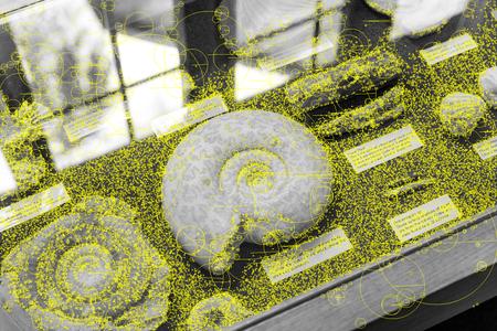
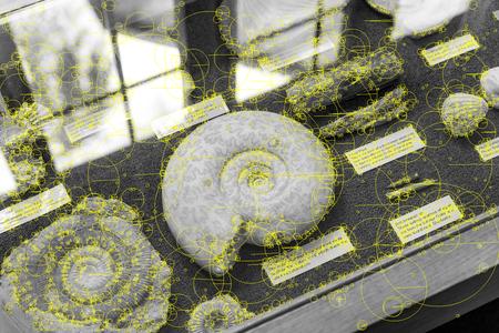
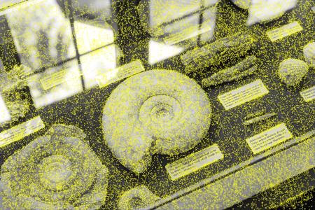
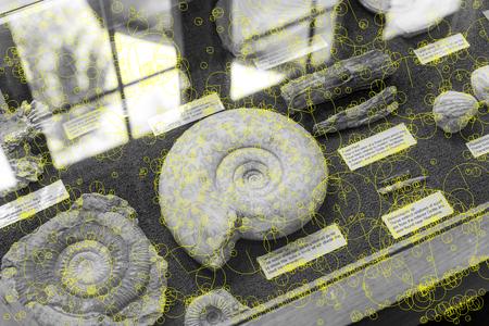
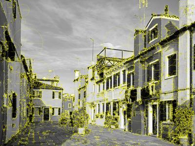
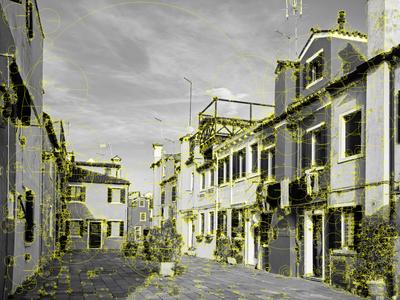
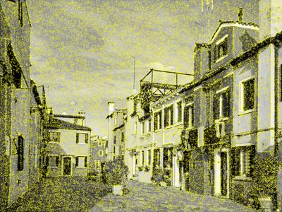
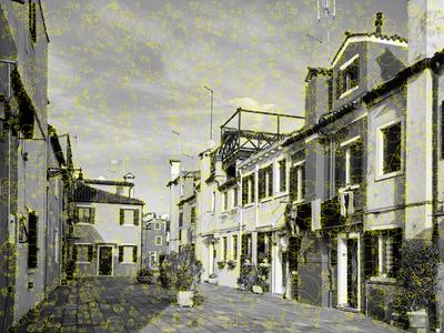
Here are some cherry picked examples to illustrate my point, as really most of the time the methods are very similar. Contrast thresholds are very small, so even the faintest features are shown. For FFD, and extra image with all the small features removed is included for visual clarity.
Click on an image to open it in full size.
Fossils (source)
Houses (source)
Mosaic (source)
This photo is shown resized both by 0.3 and 0.4 to illustrate how unreliable the detection of large blobs is with FFD. Pay attention to the big bright circle flower thingies: all SIFT variants get a good portion of them (no matter the scaling), though interestingly some of those are really quite far off location wise. FFD at 0.3x scale only shows two circles around the outermost circle, and a few more around the inner bright spot. At 0.4x scale however, all but a few of the large flowers are detected and the result actually looks really good.
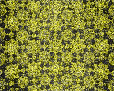
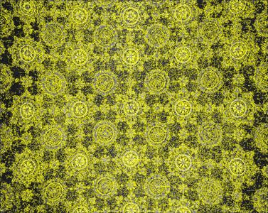


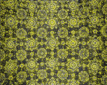
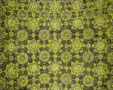
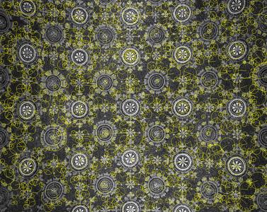
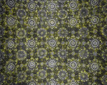
This finding is consistent over all sorts of images, the mosaic pattern just makes for an extreme example. The FFD DoG has large “blind spots” at larger features sizes that could really hold it back in tasks like registration for image search, where meaningful content is more important than tiny spots (as opposed to e.g., homography tasks, where the larger localization error makes these fairly useless).
I also think I can explain what’s happening. Recall that the main difference between SIFT and FFD scale spaces is that SIFT takes three scales for filters to double in size, while in FFD the size is doubled at every single level.
For simplicity, let’s drop to one dimension and use a single gaussian blob as our image (shown on the right). Build DoG filters \(G_{\sigma} - G_{2\sigma}\) over a range of \(\sigma\) and convolve them all with our image. The heatmap shows the filter response, reaching its maximum around \(\sigma=18\) as predicted by \(\eqref{eq:dog_sigma}\).
Marking the filter sizes where the discrete scale levels of FFD fall, the issue becomes clear:
Because of the increasingly sparse sampling of the scale space, there’s ranges of blob sizes that slip right through or become very unreliable. If you squint, the sample around \(\sigma=26\) might actually be higher than the previous and next ones in this example, marking an extremum. Even so, the amplitudes here are so tiny that interpolating the peak using second derivatives is probably a lost cause with even a bit of noise or other inaccuracies.
If I’m not completely mistaken, this problem is inherent to the FFD construction, but the original authors don’t mention anything of the sort. Instead, they seem to imply that using only three scales faster and just as good as SIFT[5:2, 14]:
[…] the proposed method does not need either upsampling or downsampling operations and thus provides good localization for the detected keypoints
[…] unlike the conventional feature detectors that split the input image into several octaves and each octave includes ‘S+3’ scale levels, we decompose the given image into just ‘N + 3’ levels that includes all the octaves and scale levels
I feel like reducing the amount work required by just “stopping early” while implying that the results of that skipped work are useless anyway is a bit cheeky honestly. Stopping after three scales is faster, yes, but it also limits you to feature sizes on the order of \(2^3=8\), while SIFT will happily find a blob spanning the entire image.
Anyway I’m tired of this now, but the logical thing to try would be to use FFD filtering for the first octave to find some of the small features that SIFT appears to miss, downsample and then proceed with regular SIFT across larger octaves. Ideally, that would improve performance on small features without the SIFT upscale and still reliably detect large ones.
Multi Kernel Descriptors
For the actual image patch descriptor, I implemented the Multi Kernel Descriptor (MKD) as proposed by Mukundan et al. [9]. The kernel framework is very general and probably applicable to many more problems, so I highly recommend reading up on the feature map construction [14], an earlier patch descriptor [1] and finally the MKD paper. The following is a short summary of these papers, starting from SIFT and working backwards.
Recall that the SIFT descriptor is essentially a histogram of the local gradient orientation over a patch. At every pixel, compute the direction along which the pixel value changes the most, and add the magnitude of that change to the appropriate histogram bin. Similarity between patches is then given by e.g., the dot product between histograms or some other distance.
A problem with histograms is that they force a discretization step very early in the pipeline, making the process very susceptible to noise, especially for sample values right on the boundary of two histogram bins. The image above demonstrates this effect: note how the big bars around \(\frac{\pi}{2}\) of the top and middle histogram just miss each other and will be lost in the element-wise multiplication. The same can be observed around \(\pm\pi\) in the middle and bottom (noisy) plot.
The kernelized descriptor approach foregoes the histogram and uses a continuous measure of similarity, which can be chosen (almost) arbitrarily. Sticking with gradient angles, the von Mises distribution is a reasonable choice. The \(\kappa\) parameter controls the width of the peak, and \(k(\theta_1, \theta_2) = \text{VonMises}(\theta_1 - \theta_2)\) shall be our kernel that measures how similar two pixels are.
That’s nice for comparing two scalars, now how do we compare over a whole patch of pixels? Easy, just compare every pixel in a patch \(\mathcal{P}\) to every other pixel in patch \(\mathcal{Q}\). That’s much more thorough than reducing everything into a histogram right away, right?
That obviously won’t work exactly as is, but here’s where the feature map trick from [2, 14] comes in. The goal is to find a clever function or feature map \(\mathcal{\psi}\) that… maps our features into a new higher dimensional space, in which linear operations (here the inner product) closely approximate a nonlinear function such as the von Mises kernel.
Kernel Trick
A staple in machine learning: we have a feature which appears too “complicated” to be captured using linear constructs, such as a nonlinear similarity kernel, or a distribution of class labels.
By finding a suitable mapping, we can represent that feature in a higher dimensional space and take advantage that the more dimensions you have, the more “complicated” linear transformations can be.
Say we have these points, can you separate the two colors by drawing a straight line?
Bet you can’t, but let’s add a dimension to make things easier and feed the samples \(x\) into some feature map. I don’t know, say:
\[ f(x) = \begin{pmatrix} 0.3x \cdot \cos{x} \\ 0.3x \cdot \sin{x} \\ \end{pmatrix} \]
Admittedly a bit contrived, but plotting these 2D vectors the problem suddenly seems much simpler:
We really want a linear measure of similarity, because it means that the sum of similarities is equal to the similarity of the sum. The latter sum here being of the feature map outputs over all pixels, which becomes the descriptor for a whole patch of pixels.
\[ \sum_{p\in \mathcal{P}} \sum_{q\in \mathcal{Q}} k(\theta_p, \theta_q) \approx {\underbrace{\sum_{p\in \mathcal{P}} \mathcal{\psi}(\theta_p)}_{\text{descriptor }\mathcal{P}}} ^\top \underbrace{\sum_{q\in \mathcal{Q}} \mathcal{\psi}(\theta_q)}_{\text{descriptor }\mathcal{Q}} \]
\(\theta_p\) is the gradient orientation of pixel \(p\) in this example. Skipping the details, we approximate \(k\) as \(\hat k\) using its truncated Fourier series i.e., a linear combination of scaled \(\sin\) and \(\cos\) basis functions. The approximated kernels look like this, with different numbers of Fourier terms retained:
MKD Fourier Coefficients
The coefficients as used in the authors’ PyTorch implementation can be reproduced as follows:
import numpy as np
from scipy.special import ive

kappa = 8
N = 4 # 3 frequencies + DC component

coeffs = [ive(0, kappa)] + [2 * ive(n, kappa) for n in range(1, N)]
coeffs = np.sqrt(np.asarray(coeffs))
print(coeffs)
ive is the modified Bessel
function of the first kind, which I’m definitely familiar with and
basically use like, all the time.
The feature map \(\mathcal{\psi} : \mathbb{R} \longmapsto \mathbb{R}^{2N+1}\) is then:
\[ \psi(\theta) = \begin{pmatrix} \sqrt{\gamma_0} \\ \sqrt{\gamma_1}\cos(\theta)\\ \sqrt{\gamma_1}\sin(\theta)\\ \vdots \\ \sqrt{\gamma_N}\cos(N\theta) \\ \sqrt{\gamma_N}\sin(N\theta) \end{pmatrix} \]
where \(\gamma_i\) is the \(i\)th Fourier coefficient of the von Mises kernel. With some trig identities, the inner product of two such vectors works out to
\[ \begin{align*} & \psi(\theta_p)^T\psi(\theta_q) \\ &= \gamma_0 + \sum_{i=1}^N \gamma_i \left[ \cos(i\theta_p) \cos(i\theta_q) \allowbreak + \sin(i\theta_p) \sin(i\theta_q)) \right] \\ & = \gamma_0 + \sum_{i=1}^N \gamma_i\cos(i(\theta_p - \theta_q)) \\ & = \hat k (\theta_p - \theta_q) \\ & \approx k(\theta_p - \theta_q) \end{align*} \]
I’m still not over this, it’s just so neat!
Earlier, we said every pixel in one patch would be compared to every pixel in the other patch, which doesn’t make much sense. Instead, the similarity of close pixels should be emphasized over that of very far away pixels. SIFT does this by dividing the patch into subpatches, each getting their own histogram (again, that discretization problem). The MKD authors instead incorporate more pixel into the similarity, once again comparing them with the von Mises match kernel (hence the “Multi Kernel” part, multiple attributes all with their own kernel).
Weighting the similarity of pixel gradients by the similarity of their coordinates in the patch amounts to just multiplying two kernel terms. Using cartesian pixel coordinates within the patch \((x_p, y_p)\) we get:
\[ \mathcal{M}(\mathcal{P}, \mathcal{Q}) = \sum_{p\in \mathcal{P}} \sum_{q\in \mathcal{Q}} k(\theta_p, \theta_q) k(x_p, x_q) k(y_p, y_q) \]
Extending the feature map trick to multiple kernels involves a Kronecker product, and the kernelized descriptor for patch \(\mathcal{P}\) is:
\[ \mathcal{V}_{cart}(\mathcal{P}) = \sum_{p\in\mathcal{P}} w_p \sqrt{m_p} \otimes \psi_{\theta}(\theta_p) \otimes \psi_x(x_p) \otimes \psi_y(y_p) \label{eq:kernel_descriptor} \]
where \(m_p\) and \(\theta_p\) are the local gradient magnitude and angle, \(x_p\) and \(y_p\) the position within the patch and \(w_p\) is a gaussian weighting that emphasizes pixels close to the patch center. This is repeated with polar coordinates as well and the resulting vectors are concatenated and postprocessed even more (see [9], it’s super interesting).
Kronecker Product
\[ \begin{equation*} \begin{pmatrix} a_1 \\ a_2 \\ a_3 \end{pmatrix} \otimes \begin{pmatrix} b_1 \\ b_2 \\ b_3 \end{pmatrix} = \begin{pmatrix} a_1b_1 \\ a_1b_2 \\ a_1b_3 \\ a_2b_1 \\ a_2b_2 \\ a_2b_3 \\ \vdots \end{pmatrix} \end{equation*} \]
Like all the other funny matrix operations and norms this probably has an actual meaning, but here it just emerges from the algebra and makes the inner product develop to the expression we need.Implementation
The formula above already looks dangerous and is a real challenge to implement efficiently. Let’s plug in numbers for the actually retained Fourier frequencies and look at the resulting vector dimensionalities (\(N\) frequencies means \(\psi(p)\) has \(2N + 1\) dimensions):
| Attribute | # Fourier Freq. | # Dimensions |
|---|---|---|
| \(x\) | \(1\) | \(3\) |
| \(y\) | \(1\) | \(3\) |
| \(\theta\) | \(3\) | \(7\) |
| Combined Cartesian | 63 | |
| \(\phi\) | \(2\) | \(5\) |
| \(\rho\) | \(2\) | \(5\) |
| \(\theta\) | \(3\) | \(7\) |
| Combined Polar | 175 |
In total that’s three nested loops for up to 175 components, summed over a \(32\times 32\) patch. Note that the coordinate embeddings are always the same and may be precomputed, the \(\psi\)-embedded gradient orientation is the actual input vector. That makes for a combinatorial explosion of possible implementations and parallelization strategies. A non-exhaustive list of considerations:
- Parallelize over the 7 input dimensions, distributing them over workgroups
- Partially parallelize the input dimensions and a subset of the position embeddings, say 1 input dimension and 4 position dimensions per workgroup
- Divide the input patch, and have 1 (or more) workgroup per sub-patch, then combine (sum) the partial results
- Any combination of the tiling/blocking schemes above
- At any level in the nested loops, results for the next iteration of the outer loop can be discarded and recomputed or (partially) stored. Registers are scarce and memory accesses are slower than recomputing, except sometimes they’re not.
- If one thread processes multiple pixels, 175 partial sums either have to be accumulated or reduced among multiple threads. We can update partial results in shared memory every iteration, or every \(M\) iterations and keep \(M\) results in registers instead.
And on and on… Beyond a bit of intuition, I think the only way to find out is to try them all and measure. Also, the cartesian and polar versions with 63 and 175 dimensions respectively behave quite differently obviously, so they’re optimized separately. That’s what I did for my machine (Ryzen 7840HS, RDNA3) until I got bored and what I have is pretty good, but those results may not be applicable to other platforms.
Beyond tedious trial and error, there’s one trick I am very pleased with and that actually had an impact. Recall that every pixel is characterized by the local gradient, but also its position within the patch encoded as either cartesian coordinates in \([-1, 1]\) or polar coordinates \(\phi \in [-\pi, \pi]\) and \(\rho \in [0, 1]\). There are obvious symmetries here: \(x\) is constant within a column, \(y\) within a row (and with a sign flip there’s one more symmetry), \(\rho\) is symmetric around the origin, and \(\phi\) is similar between quadrants.
It just so happens that the \(\psi\) feature maps are also nicely symmetric, since the components are just scaled sines and cosines.
Working it out for all the feature maps and coordinate systems, we see that every component of the various \(\psi\) mappings is symmetric over the four quadrants, save a few sign flips or \(\pm \pi\). That means every pixel in the patch has three buddies that share a lot of computation, which we definitely want to take advantage of.
We can do that by appropriately rearranging
the pixels of the input patch (swizzling) such that corresponding
samples from the four quadrants end up next to each other. Now we can
work with four samples at a time (using wide loads like
gather4), compute embedding coefficients as scalar values
and broadcast
them to vectors at the last second. While this does free up a couple
of registers and give the compiler more room to optimize, loading and
processing four samples obviously requires four times as many registers
in other places, taking occupancy down to around 60%. In my benchmarks
that was still faster than my previous attempts, but I’m certain you
could do better given enough time and perseverance. I’d also love to see
how this works out on a CPU with real SIMD and instruction level
parallelism, the benefits there might be even greater.
Some conclusions I think I can draw:
- Splitting a workload over multiple workgroups at the cost of a reduction pass afterwards is almost never worth it. In all this work, there has not been a single case where it helped in any way, usually it made things worse. Vulkan is unfortunately fundamentally limited in that regard.
- Vector registers are too precious to do anything smart like register blocking. In the cartesian case I’m getting away with it and it might be a tiny bit better than always hitting shared memory, but the polar version can’t spare any registers anywhere.
- Chasing occupancy can become counterproductive at some point. If you’re not wasting registers and the computation just involves lots of values and results, bending over backwards to use fewer registers rarely leads to wall clock time savings.
The rest of the implementation isn’t too special, so I’ll skip it here.
Descriptor Extraction Performance
The setup is the same as earlier, but this time the image size is fixed and the number of features is the variable (just stop when the maximum number is reached, no ranking or anything going on).
You’ll notice that MKD is much more expensive than SIFT (almost free on CPU, still cheap on GPU), so filtering features to process further already becomes quite important even before any matching or retrieval is done. As far as I’m aware, the PyTorch implementation in Kornia is the only other public implementation, so I don’t have anything to compare my results to.
Evaluation
I don’t have anything worthwhile to present here and refer to Dmytro Mishkin, who doubts that any of the microbenchmarks and metrics commonly used to evaluate descriptors and matching performance are of much use at all. You need to evaluate on a specific task from start to finish, for example on the COLMAP[12] reconstruction benchmark. Running these is a real project though, for which I have neither the time nor hardware unfortunately. I have run other homography benchmarks like HPatches (which is a bit too easy these days), and the gist is that (Root)SIFT is generally a tiny bit better, though margins are small enough that tweaking the protocol and aggregate statistics could really back up any result you want.
MKD is almost certainly a stronger descriptor in general than SIFT[9:12–14], but that doesn’t say much about the performance on blob-like features only, which are the only ones we get with DoG detectors. I’m pretty sure it’s the quality (number, repeatability) of detected features that’s holding us back, not the descriptors.
The core principles of the SIFT DoG detector and FFD are the same, so there’s no a priori reason to assume one to drastically outperform the other, and anecdotally that seems to be true. They reliably detect high contrast blobs and become spotty at similar levels of difficulty. FFD did slightly better on a (proprietary) dataset of flat images with mostly fine details only, while SIFT is noticeably better with large features and faired better in my HPatches experiments. I definitely have no conclusive answer here, though my hunch is that FFD’s troubles with larger blobs are not offset by its ability to resolve tiny grains better.
Some of the results presented in the FFD paper (p. 11-13) seem quite surprising with that in mind. The numbers show it competing with and often times beating big, trained models like SuperPoint[3] or D2Net[4] which are definitely in different weight classes than a bit of smart Gaussian filtering.
While I don’t claim to have the expertise to comment on these comparisons, I am confident enough to say that the performance analysis in Section 4.7 is incorrect. The authors essentially count the number of arithmetic operations required for SIFT DoG and their method to show that it’s 20 times faster, completely ignoring the fact that memory latency is the obvious limiting (and really the only relevant) factor here. My laptop can do triple digit billions of floating point operations per second, and by that logic wrangling a few ten million pixels should be almost negligible. It’s not though, because touching every pixel of an image just takes an amount of time that you can do very little about.
Moreover, even counting filter taps is a very simplistic model that doesn’t reflect how actual computers work: fetching two pixels does not take twice the time as one, if only because of the fact that cache lines exist and are usually 32 or 64 bytes. Modern memory subsystems are incredibly complex (even more so on GPUs) for an \(mx+b\) model to be all too useful. Add to that the sparsity of FFD’s filters, and the general statement of “X is faster than Y” without specifying hardware and implementation characteristics just becomes nonsensical.
The reported experimental results are all the more interesting, since they confirm that \(20\times\) claim: on a Xeon 6130, a \(800\times 640\) image takes:
- 500ms for SIFT
- 159ms for SURF
- 2.7s for HarrisZ
- 12s for TILDE
- 29ms for FFD
I do think a performance benchmark where the timings for one task span three orders of magnitude merits a little acknowledgement or even explanation for that, because as is these values seem… peculiar. Moving on to the GPU measurements, TCDET on a Tesla P100 is reported to take 4.1 seconds, while the original TCDET paper[15:6.1] reports 10 frames per second on an older Titan X, at higher resolution. Since there’s no code available, the smell test is all we have and I’m not sure if those numbers do well there.
What Now
While this project was fun and educational, I have no actual use for it so I think I’m done with it for the time being. There’s a ton of work left obviously, but that’s mostly cleanup/robustness/fixes and optimizations for e.g., the convolution shaders which just becomes tedious busywork at some point.
Some of the more interesting improvements could be:
- LightGlue[7] feature matching: nearest neighbor search is terrible, and replacing it with a bit of trained smartness drastically improves SIFT performance at (hopefully) acceptable computational cost.
- MKD postprocessing: Currently, the 238 vectors (32 bit float) are cut to 128 after a reprojection learned from labeled match/no-match pairs (PCA with extras). Adding some nonlinearity (and/or more layers?) would be interesting to try. Also matryoshka-style vectors (components ordered by “importance”, so you can first match 4 dimensions only and quickly filter out promising match candidates), 8/4/1 bit quantizations.
- Dense MKD extraction: no blob detector, just take patches all over the image, for things like image search engines.
The project repo contains the webcam demo from the video up top (Linux only). It’s GPLv3 licensed and in a mostly workable state for anyone who wants to play with, or even has a real use for it (that would probably motivate me to work more on this too!).
